Interpreting multivariable regression coefficients in observational clinical research: The Table 2 fallacy

ABSTRACT

Multivariable regression tables are common in observational clinical research, but their coefficients are often over-interpreted. A model built to estimate the effect of 1 exposure may also report coefficients for age, sex, comorbidities, behaviours, and other adjustment variables. These additional rows are frequently read as independent risk factors, even when the analysis was not designed to estimate their effects. This is the Table 2 fallacy. The problem is not the use of adjustment, but the interpretation of adjustment terms as if each were a separate causal estimate. In this commentary, we use a directed acyclic graph and a single worked example to show why the coefficient for the exposure of interest can answer the intended clinical question, while coefficients for adjustment variables may not represent clinically actionable effects. We also show how similar errors arise when interaction terms are interpreted as causal. Authors should specify the target estimand (the causal effect the analysis is designed to estimate) and exposure, choose adjustment variables from the assumed causal structure, interpret only the exposure coefficient, and fit a separate model for each further question. We set out red flags, recurring pitfalls, and questions to ask of any risk-factor table. A regression table is not a menu of modifiable risks. An association is clinically actionable only when the study was designed to support that interpretation.

An adjusted regression table can make a modelling decision look like a clinical finding. In many observational studies, the row of interest is the exposure—the comparison the model was built to estimate. The other rows often list age, sex, comorbidities, behaviours, and other variables included to control confounding. Because all rows are displayed in the same format, they are easily read as equivalent clinical effects. That reading is often wrong.

Statistical results have long been vulnerable to over-interpretation. Over the past decade, sustained efforts have improved how clinical researchers report statistical findings. The American Statistical Association has cautioned against treating a P value threshold as the basis for scientific conclusions,^1,2 and others have urged that statistical significance not be treated as a statement of truth.³ Several journals now discourage, or decline to publish, P values in favour of effect estimates and confidence intervals (CIs),^4-6 while estimation graphics have been promoted to make both the estimate and its uncertainty visible.⁷ A similar case for CIs was made in Singapore in 2010.⁸

These reforms are important, but they leave a more basic problem untouched—an estimated coefficient may be accompanied by a CI and still be given the wrong causal interpretation. In clinical research, observational studies often aim to answer causal questions using multivariable regression models. An effect estimate and CI for the exposure of interest are reported, alongside coefficients for variables included for adjustment. The issue is not adjustment itself, but a habit that remains common in observational clinical research—reading every coefficient in the adjustment model as if it were a causal effect. Presenting the coefficient for every adjustment variable within a table, and interpreting each as an independent effect estimate, is referred to as the Table 2 fallacy, named for the table in which it characteristically appears.⁹

The fallacy arises because a multivariable model is usually intended to answer a specific clinical question. For example, a study may seek to estimate the effect of rheumatoid arthritis on cardiovascular risk while adjusting for age, smoking, hypertension, and diabetes. The adjustment variables are included to obtain a less biased estimate of the effect of rheumatoid arthritis; they are not necessarily included to estimate their own effects on cardiovascular risk. This can be understood using a directed acyclic graph, a diagram in which arrows represent assumed causal relationships between variables (Fig. 1).¹⁰ In such a framework, the total effect of an exposure is its overall influence on the outcome through all causal pathways. Some of these pathways may pass through intermediate variables, known as mediators (steps on the causal path from exposure to outcome). To estimate the exposure’s effect without confounding, investigators adjust for variables that influence both the exposure and the outcome.¹⁰ The adjustment set is chosen to answer a single causal question: the effect of the exposure on the outcome. Consequently, although the adjustment variables’ coefficients appear in the same regression table, they are adjustment terms, not separate causal estimates.

Fig. 1. Directed acyclic graph for the worked example.

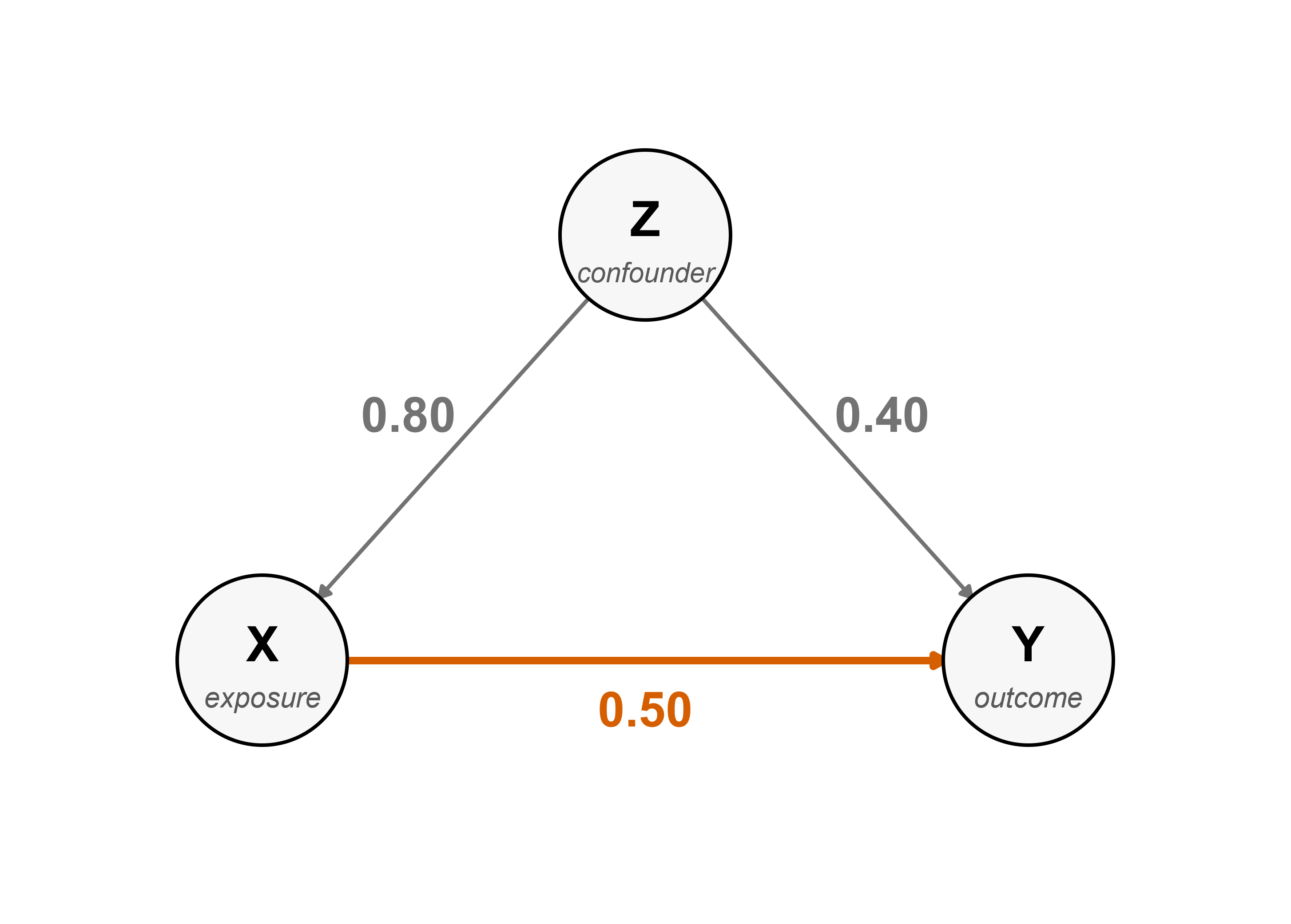The exposure X is rheumatoid arthritis, the outcome Y is cardiovascular risk, and the confounder Z is smoking. Smoking causes both rheumatoid arthritis and cardiovascular risk, while rheumatoid arthritis also causes cardiovascular risk; Z is therefore adjusted for because it confounds the X–Y relationship. Arrows are labelled with the data-generating coefficients used in the simulation: Z→X = 0.8, the direct Z→Y effect = 0.4, and the target X→Y effect = 0.5 (highlighted). Data were generated from a linear model with standard normal errors (Supplementary Appendix S1).

Consider the same example, simplified to a single confounder: a model for the effect of rheumatoid arthritis on cardiovascular risk, adjusting for smoking, a cause of both (Fig. 1). In plain terms, smoking is included to help estimate the effect of rheumatoid arthritis, not to answer a separate question about smoking itself. In this model, the coefficient for rheumatoid arthritis can be read as an estimate of its total effect on cardiovascular risk in the simplified causal diagram, because there is no mediator between rheumatoid arthritis and cardiovascular risk. The coefficient for smoking is different. Although it may appear to represent smoking’s effect on cardiovascular risk, it actually represents smoking’s effect after accounting for rheumatoid arthritis. In other words, it estimates only the part of smoking’s effect that is not explained by its influence on rheumatoid arthritis. If smoking increases cardiovascular risk partly by increasing rheumatoid arthritis, then the adjusted smoking coefficient understates smoking’s total effect.

Estimating smoking’s total effect is a separate causal question. To answer it, rheumatoid arthritis should not be included in the adjustment set, because it lies on the causal pathway from smoking to cardiovascular risk. The model would instead need to adjust for confounders of smoking itself.¹¹ In this simplified example, there are none, so a model containing smoking alone would be sufficient, but only because smoking is assumed to have no confounders here, not as a general rule. A different question, such as separating smoking’s direct effect from the part acting through rheumatoid arthritis, would require methods designed for mediation. The fitted model and estimates are provided in the Supplementary Appendix S1.

The same reasoning applies when a table suggests that the exposure effect differs between groups. Suppose a study asks whether rheumatoid arthritis raises the risk of an adverse cardiovascular outcome, adjusts for smoking, and includes a rheumatoid arthritis × smoking interaction term to allow the rheumatoid arthritis effect to differ between smokers and non-smokers. The results table suggests the association is stronger in smokers than in non-smokers. It is tempting to read this causally: that smoking worsens the effect of rheumatoid arthritis, and that smoking cessation would reduce the excess risk. Strictly, however, this table has only asked whether the rheumatoid arthritis effect differs across smoking groups. That is effect modification—how the effect of 1 exposure varies across levels of another variable. It is not the same as estimating the joint causal effect of both rheumatoid arthritis and smoking. To answer that second question, smoking would need to be treated as a second exposure, with its own causal question and sufficient adjustment set.¹² The difference between smoking groups is represented by an interaction term, but that term is still part of the model, and on its own, it describes effect modification, not a causal interaction. It should not be read causally unless the causal question and the adjustment set required to answer it have been specified. Interpreting it causally is therefore another manifestation of the Table 2 fallacy, even when the main estimate for rheumatoid arthritis is valid.

The problem becomes clearer with unmeasured factors. Smokers may differ from non-smokers in ways that are hard to capture completely, including diet, physical activity, and access to preventive care. These factors may influence both smoking and cardiovascular risk. Although adjusting for smoking may suit the rheumatoid arthritis question, smoker and non-smoker comparisons are still made within the structure the adjustment model creates. Apparent differences between these groups may therefore reflect not only genuine effect modification but also residual confounding or modelling artefacts. In the extreme, the entire apparent difference between smokers and non-smokers could reflect such unmeasured factors rather than any effect smoking cessation would alter; the coefficients for smoking, age, sex, and their interactions remain quantities the analysis was never designed to interpret causally.

The error is not remedied by a change of wording. Calling these estimates “independent associations” still invites each row to be read as a distinct effect, and terms such as “potential risk factor” and “predisposing factor” further imply an actionable, quasi-causal relationship.^13,14 The causal interpretation then often reappears in the discussion, through mechanistic explanations or recommendations for intervention. A disclaimer of “association only” relocates the fallacy rather than resolving it.

Several steps help to avoid the Table 2 fallacy. First, define the purpose of the analysis. Observational data can be used to describe patterns, build prediction models, or answer causal questions. If the aim is description, report descriptively. If the aim is prediction, evaluate prediction performance rather than interpreting coefficients as intervention effects. If the aim is causal inference, specify 1 exposure, 1 outcome, and 1 target estimand. The exposure estimand is interpretable as causal only if the causal question is well defined and the adjustment set is sufficient; it must control confounding without adjusting for mediators or colliders of the exposure–outcome relationship. The remaining variables are used for adjustment, not to be read as a menu of risk factors. If another variable seems interesting in its own right, treat it as a distinct question, with its own causal diagram, its own sufficient adjustment set, and its own model. A well-presented table makes this explicit (Table 1): the exposure is set apart and interpreted, while the adjusted variables are grouped and flagged as included for confounding control, not as separate causal effects.

Table 1. Adjusted risk ratios from a hypothetical, illustrative multivariable model for incident cardiovascular events, with each coefficient grouped by its causal role. The rheumatoid arthritis exposure is represented here as graded inflammatory disease activity, to illustrate a multi-level exposure.

CI: confidence interval; RR: risk ratio

^a The exposure block is the causal contrast the model was designed to estimate, using a pre-specified adjustment set derived from the causal diagram; it is interpretable only when that adjustment set is sufficient and contains no mediator or collider of the exposure. Its category contrasts form part of the same exposure definition and should be interpreted together.
^b The adjustment variables are included for confounding control, not because their coefficients are target effects. Each variable has its own causal structure and would require its own adjustment set before its coefficient could be interpreted causally. Treating these coefficients as independent risk factors is the Table 2 fallacy.
^c Adjustment set: sex, age, smoking, lower income, diabetes mellitus, hypertension.
^d Risk ratios are collapsible: when there is no confounding and no effect modification on the risk ratio scale, the marginal risk ratio equals the stratum-specific risk ratio. For non-collapsible measures such as the odds ratio and hazard ratio, conditional and marginal estimates may differ even in the absence of confounding, mediation, or effect modification, for reasons unrelated to the Table 2 fallacy.^15,16

Second, pre-specify the adjustment set from the assumed causal structure, rather than selecting adjustment variables by stepwise procedures or statistical significance. These procedures may be useful for prediction, but they do not define a causal adjustment set. A variable may be needed for confounding control even if it is not statistically significant, while a statistically significant variable may be inappropriate to adjust for if it is a mediator or a collider (a variable influenced by both the exposure and the outcome, which adjustment can bias).¹⁷

Third, present the primary result as an estimation graphic rather than a dense coefficient table in which every variable invites a causal reading. The graphic shows the single-adjusted exposure effect with its full uncertainty rather than a significance test; in the worked example, the smoking-adjusted outcome is plotted for 2 groups, with the adjusted effect and its bootstrap distribution shown alongside (Supplementary Fig. S1). The same principle of reporting the adjusted effect with its uncertainty applies whatever the effect measure (mean difference, risk ratio, or risk difference).

Finally, because no observational adjustment can be assumed complete, the extent of residual confounding should be quantified, for example with an E-value, which indicates how strong an unmeasured confounder would need to be to explain away the observed exposure effect.¹⁸ Box 1 lists red flags, recurring pitfalls, and questions a reviewer can ask of any risk-factor table.

Box 1. Spotting the Table 2 fallacy: Red flags, common pitfalls, and questions for reviewers.

None of these steps is demanding, yet together they turn a regression table from a list of numbers into a clearly defined estimate whose causal interpretation can be assessed.

CONCLUSION

The Table 2 fallacy arises when coefficients included for adjustment are interpreted as separate causal effects. Avoiding it requires a clearly defined exposure, the effect to be estimated, the underlying assumptions, and the variables needed for adjustment. This principle applies to every table reporting estimates from a multivariable model: interpret the effect the analysis was designed to estimate, and treat the remaining coefficients as adjustment terms rather than findings in their own right. The distinction requires no new software or larger sample, only the habit of asking what causal question each coefficient answers and whether the study design can answer it.

Supplementary materials

Fig. S1. Estimation graphic for the adjusted exposure effect (illustrative simulated data).
Appendix S1. R code for the simulation.

Acknowledgments

John Rong Hao Tay is supported by the Singapore National Medical Research Council Research Training Fellowship (RTF24jan-0007). Nasir Z Bashir is supported by the Wellcome Trust (322777/Z/24/Z).

REFERENCES

1. Wasserstein RL, Lazar NA. The ASA statement on p-values: context, process, and purpose. Am Stat 2016;70:129-33.
2. Putt ME. Assessing risk factors with information beyond P value thresholds: Statistical significance does not equal clinical importance. Cancer 2021;127:1180-5.
3. Amrhein V, Greenland S, McShane B. Scientists rise up against statistical significance. Nature 2019;567:305-7.
4. Trafimow D, Marks M. Editorial [Banning null hypothesis significance testing procedures]. Basic Appl Soc Psychol 2015;37:1-2.
5. Lang JM, Rothman KJ, Cann CI. That confounded P-value. Epidemiology 1998;9:7-8.
6. Hayat MJ, Staggs VS, Schwartz TA, et al. Moving nursing beyond p < 0.05. Res Nurs Health 2019;42:244-5.
7. Ho J, Tumkaya T, Aryal S, et al. Moving beyond P values: Data analysis with estimation graphics. Nat Methods 2019;16:565-6.
8. Tan SH, Tan SB. The correct interpretation of confidence intervals. Proc Singap Healthc 2010;19:276-8.
9. Westreich D, Greenland S. The Table 2 fallacy: Presenting and interpreting confounder and modifier coefficients. Am J Epidemiol 2013;177:292-8.
10. Greenland S, Pearl J, Robins JM. Causal diagrams for epidemiologic research. Epidemiology 1999;10:37-48.
11. Tennant PWG, Murray EJ, Arnold KF, et al. Use of directed acyclic graphs (DAGs) to identify confounders in applied health research: Review and recommendations. Int J Epidemiol 2021;50:620-32.
12. VanderWeele TJ. On the distinction between interaction and effect modification. Epidemiology 2009;20:863-71. Erratum in: Epidemiology 2011;22:752.
13. Schisterman EF, Cole SR, Platt RW. Overadjustment bias and unnecessary adjustment in epidemiologic studies. Epidemiology 2009;20:488-95.
14. Tay JRH, Cooray U. Letter to Editor for “Potential predisposing features of external cervical resorption: An observational study (Patel et al., 2025)”. Int Endod J 2025;58:797-8.
15. Greenland S, Robins JM, Pearl J. Confounding and collapsibility in causal inference. Stat Sci 1999;14:29-46.
16. Hernán MA. The hazards of hazard ratios. Epidemiology 2010;21:13-5.
17. Harrell FE Jr. Regression Modeling Strategies: With Applications to Linear Models, Logistic and Ordinal Regression, and Survival Analysis. 2nd ed. Cham: Springer; 2015.
18. VanderWeele TJ, Ding P. Sensitivity analysis in observational research: Introducing the E-value. Ann Intern Med 2017;167:268-74.